What Chance Looks Like – A Fine-Tuned Critique of Richard Carrier (Part 2)

Last time, we looked at historian Richard Carrier’s article, “Neither Life nor the Universe Appear Intelligently Designed”. We found someone who preaches Bayes’ theorem but thinks that probabilities are frequencies, says that likelihoods are irrelevant to posteriors, and jettisons his probability principles at his leisure. In this post, we’ll look at his comments on the fine-tuning of the universe for intelligent life. Don’t get your hopes up.

Simulating universes

Here’s Carrier.

Suppose in a thousand years we develop computers capable of simulating the outcome of every possible universe, with every possible arrangement of physical constants, and these simulations tell us which of those universes will produce arrangements that make conscious observers (as an inevitable undesigned by-product). It follows that in none of those universes are the conscious observers intelligently designed (they are merely inevitable by-products), and none of those universes are intelligently designed (they are all of them constructed merely at random). Suppose we then see that conscious observers arise only in one out of every universes. … Would any of those conscious observers be right in concluding that their universe was intelligently designed to produce them? No. Not even one of them would be.

To see why this argument fails, replace “universe” with “arrangement of metal and plastic” and “conscious observers” with “driveable cars”. Suppose we could simulate the outcome of every possible arrangement of metal and plastic, and these simulations tell us which arrangements produce driveable cars. Does it follow that none of those arrangements could have been designed? Obviously not. This simulation tells us nothing about how actual cars are produced. The fact that we can imagine every possible arrangement of metal and plastic does not mean that every actual car is constructed merely at random. This wouldn’t even follow if cars were in fact constructed by a machine that produced every possible arrangement of metal and plastic, since the machine itself would need to be designed. The driveable cars it inevitably made would be the product of design, albeit via an unusual method.

Note a few leaps that Carrier makes. He leaps from bits in a computer to actual universes that contain conscious observers. He leaps from simulating every possible universe to producing universes “merely at random”. As a cosmological simulator myself, I can safely say that a computer program able to simulate every possible universe would require an awful lot of intelligent design. Carrier also seems to assume that a random process is undesigned. Tell that to these guys. Random number generators are a common feature of intelligently designed computer programs. This argument is an abysmal failure.

How to Fail Logic 101

Carrier goes on …

If every single one of them [conscious observers in simulated universes] would be wrong to conclude that [their universe was intelligently designed], then it necessarily follows that we would be wrong to conclude that, too (because we’re looking at the same evidence they would be, yet we could be in a randomly generated universe just like them).

In other words, if we are in randomly generated universe, then we observe a life-permitting universe. We observe a life-permitting universe. Thus, we are in a randomly generated universe. This is a textbook example of affirming the consequent, a “training wheels” level logical fallacy. That the evidence is consistent with a hypothesis doesn’t mean that the hypothesis must be true.

Don’t Play Poker Like This

It simply follows that if we exist and the universe is entirely a product of random chance (and not NID), then the probability that we would observe the kind of universe we do is 100 percent expected. … The conscious observers in that universe [the only existent universe, just by chance finely tuned to produce intelligent life] would see exactly all the same evidence [as in a multiverse]… The evidence simply always looks exactly the same whether a universe is finely tuned by chance or by design – no matter how improbable such fine-tuning is by chance. And if the evidence looks exactly the same on either hypothesis, there is no logical sense in which we can say the evidence is more likely on either hypothesis. Think of getting an amazing hand at poker: whether the hand was rigged or you just got lucky, the evidence is identical. So the mere fact that an amazing hand at poker is extremely improbable is not evidence of cheating.

False. Obviously false.

Think for half a second about the poker example. Suppose I am dealing, and I deal myself a Royal flush. “No evidence of cheating there”, you think, “since a Royal flush looks the same whether he’s cheating or not”. Then it happens again. And again. It happens 20 times in a row. Unless you’ve crippled your ability to calculate probabilities by subscribing to finite frequentism, you know that the probability of this happening with a fair dealer is 1 in . However, if the extreme improbability of an amazing hand at poker is not evidence of cheating, then neither is the extreme improbability of 20 amazing hands. “Whether the hands were rigged or he just got lucky, the evidence is identical”, you think. So 20 Royal flushes in a row is not evidence of cheating. If Carrier actually believes that, then I’d love to play poker with him.

Here’s a free lesson on how to use Bayes’ theorem to analyse this scenario. If the prior probability that I would cheat is , the probability of getting a sequence of fairly-dealt Royal flushes is , and the probability of R given that I am cheating is , then the probability that I am cheating is, by Bayes’ theorem

.

As more Royal flushes are dealt, gets smaller, gets larger and it becomes more probable that I am cheating. This is Bayes’ theorem 101. More than that, it’s nose-on-your-face obvious that the guy winning every hand is more likely to be cheating. Whose probability intuitions are that bad?!

When the Evidence “Looks the same”

Carrier says that “if the evidence looks exactly the same on either hypothesis, there is no logical sense in which we can say the evidence is more likely on either hypothesis”. Nope. Repeat after me: the probability of what is observed varies as a function of the hypothesis. That’s the whole point of Bayes theorem.

For example, the cheating hypothesis and the fair-dealer hypothesis are equally able to put a Royal flush on the table. The evidence looks exactly the same. Given that you cheat in order to win, a Royal flush is much more likely to be dealt if the dealer is cheating. So the evidence is more likely on the cheating hypothesis. This is so blindingly obvious it would usually go without saying. The same evidence E can have different probabilities depending on the hypothesis. The likelihood of E given two different hypotheses and will in general be different, . That’s the whole frigging point of likelihoods! That’s why we collect evidence! That’s how we test theories! That’s how posterior probabilities update given new evidence!

The Firing Squad Machine

Let’s take a look at Carrier’s version of the firing squad analogy. You are placed in a room with a mystery machine that fires bullets. Having fired a large number of bullets, each in a different, seemingly random direction, you are still alive. What should we conclude about the machine?

We know that,

Fn = n bullets have been Fired (n > 0).

M = all the bullets have Missed me.

L = I am still Living

(With a slight abuse of notation, assume any relevant background information B in each probability below).

Two theories we could consider are,

D = the machine is Designed to ensure my survival

I = the machine is Indifferent to my survival

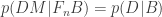
Assume for simplicity that the bullets are cyanide-coated so that any hit will kill. Then

for all n.     (8)

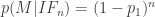
As above, we can prove fairly easily that, given that I am alive, all the bullets must have missed me regardless of whether the machine is designed or indifferent,

for all n.     (9)

So, given what I know (in particular, M), the probability that I live is one, regardless of whether the machine is designed or indifferent. Does it follow that I have no information at all as to the design of the instrument? Intuitively, I must. If the machine fires 1 million bullets, so that the walls of the room are riddled with bullets except for a perfect outline of my silhouette, surely we’d start to suspect that the machine wasn’t the random killing machine we’d feared. Bayes’ theorem backs this up. We can calculate the ratio of the posterior probabilities of our two theories,

(Bayes’ theorem)

(by 9)

(Bayes’ theorem)

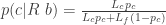
The first term is the ratio of the likelihoods. How likely is it that all the bullets would miss me, given n bullets were fired and the machine is either designed to keep me alive or designed indifferently? Very roughly, if the machine is designed for life then we expect it to do its job, . If the machine shoots bullets indiscriminately, then in the absence of any more information about the machine we can assume that there is some probability that I would be hit on any given shot. Then, , which approaches zero as . Thus, as the number of misses increases, the probability of D relative to I approaches one.

Bayes’ Theorem Omits Redundancies

Something to note from the discussion above. While L is not given in the likelihoods, it is given in the posterior, as the sequence of equals signs show. Thus, the fact that L does not appear in certain terms in the equation does not mean that we are ignoring L, or reasoning as if we didn’t know L, or pretending that L doesn’t count. Put another way – just because something is known, doesn’t mean that it is taken as given in every term in our calculation of the posterior. If that confuses you, read this.

This applies more generally. The equations above show that, given any theory , and any collection of known facts ,

does not imply .

This is true, even though , i.e. that is “100 percent expected” given A, and A is known. Bayes’ theorem is perfectly able to handle redundancy in the data.

It follows that Carrier’s “formal proof” of his central argument in footnote 23 fails. Applying this to fine-tuning, let:

f = Finely tuned universe

o = intelligent Observers exist

NID = Non-terrestrial Intelligent Design

b = background knowledge

All that follows from the anthropic principle – that observers will observe that they exist in a life-permitting universe – is that we need not condition on both and when testing the hypothesis NID. It does not follow that NID and ~NID are equally probable given the evidence. The probability of ~NID depends on the likelihood p(f|~NID b), where is not part of the background. When we argue from the small probability of a life-permitting universe “constructed at random”, we aren’t pretending that we don’t know whether we exist, or that this fact doesn’t count. See also this post regarding Carrier’s discussion of Collins – if your posterior changes when you move statements from e to b then you’re doing it wrong.

Carrier’s Account of the Firing Squad Machine

Having seen the Bayesian account above, let’s see how Carrier analyses the machine.

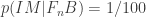
Suppose we knew in advance that 1 in 4 such machines was rigged to miss, and that the chance of their missing by accident was 1 in 100. Then we would infer design, because in any cohort of 1,000 victims, on average 250 will survive by design and only 10 will survive by chance, so if you are a survivor your prior odds of having survived by chance are 10 in 260, or barely 4 percent.

In our notation, the prior probability of a rigged machine . However, the second claim is not the prior probability that the machine aims at random, . Rather, it is the probability that the machine aims at random and misses an unspecified number of shots, for some n. So we should be comparing to , though since we can assume the likelihood , . It follows that 10 in 260 is the posterior of , not the prior. Even this assumes that D and I are exhaustive. (Also, they aren’t odds – odds are the ratio of probabilities, 10 to 250. If I’d given him any marks so far, he’d have lost one there for not knowing the basic vocabulary of probability.)

No sign of probability theory competence there, but let’s keep looking.

But suppose you knew in advance that only one in four results was a product of design, and the others were chance. Then in any cohort of a thousand victims you will still know there are on average ten survivors by chance, but you will also know that for every survivor there is who survived by design, there more will have survived by chance, so you know that there can be, on average, only three who survived by design – so if you are a survivor, your odds of having survived by chance are still three in four or 75 percent. In this case, you shouldn’t conclude design, and that’s even knowing the odds of having survived by chance are 1 in 100.

Lesson 1: 78 words in a sentence is too many, especially if it includes the conjunction “so” twice, one “but” and an ill-advised em dash.

The reason why Carrier’s confusion between prior and posterior in the previous paragraph is more than a notational blunder is that he now tries to change the posterior. We saw in a previous post why simply announcing a posterior probability is backwards, unBayesian and unrealistic. But now it’s even worse. Carrier effectively announces that the posteriors have a certain ratio . Even worse, he says that this holds “in advance”! They’re posteriors! Posterior means “coming after”. If you’re specifying posterior probabilities before the evidence comes in then you’re either match-fixing or have no frigging clue what you’re talking about.

As in the previous post, we can calculate the probabilities that Carrier is assuming behind the scenes. Since , it must be that . Carrier has simply lowered the prior on the theory he wants to discount. If you can do that, you can believe anything you like.

Conclusion

Here’s why this matters, and with this Carrier’s essay finally bleeds to death.

[In] our background knowledge, we have no evidence that the frequency of very improbable events (not already caused by known life) being products of NID is anything higher than 25 percent. It doesn’t matter how improbable any of those events are. … Thus we cannot conclude that the probability that the universe is a product of NID is anything higher than its prior probability of 25 percent.

The whole point of Carrier’s analysis of the firing squad machine was that you can ignore the prior only in the case where you, clairvoyantly, specify the posterior. So Carrier’s argument from background evidence and the prior probability misses his own point. Unless Carrier can magically pull the posterior probability of NID from his posterior, he’s going to have to deal with Bayes’ theorem. The posterior is only equal to the prior if the likelihood of NID is equal to the likelihood of ~NID. As we saw above, this does not follow from the anthropic principle. Carrier’s argument fails.

The probability of ~NID depends on the probability of a life-permitting universe existing “by chance”. If it is very small, as fine-tuning suggests, then the probability of ~NID may also be very small. Carrier’s compendium of elementary logical and probabilistic blunders does nothing to turn back the force of the fine-tuning argument. If you want to read a decent critique of the argument, try Sean Carroll, Paul Davies, Alex Vilenkin, Leonard Susskind, Bradley Monton, or perhaps someone who actually understands physics, cosmology and probability.

Advertisement